03-Convex-Optimization-Problems

This is the third notebook of the series going through Convex Optimizaion. The topics here are following MOOC Convex Optimization course by Stephen Boyd at Stanford.

Convex Optimization in standard form

A convex optimization problem is one of the form:

\[\begin{align} \text{minimize }& f_0(x)\\ \text{subject to }& f_i(x) \leq 0, i=1,\dots,m\\ & a_i^Tx=0 , i=1,\dots,p\\ \end{align}\]

where $f_0,\dots,f_m$ are convex functions and equality constraints are affine.

• feasible set of a convex optimization problem is convex: \(D=\bigcap_{i=0}^m \textbf{dom }f_i \cap \bigcap_{j=0}^p \textbf{dom }h_j\)

Local and global optima

For any convex optimization problem, any locally optimal point is also (globally) optimal.

Suppose:

\(f_0(x)=\text{inf }\{f_0(z)|z \text{ feasible }, \parallel z-x \parallel_2 \leq R\}\) for some $R$. Suppose $x$ is not globally optimal. Then there is a feasible $y$ such that $ f_0(y)<f_0(x) $ and \(\parallel y-x\parallel_2>R\). Now consider the point $z$: $z=(1-\theta)x+\theta y, \theta=\frac{R}{2\parallel y-x\parallel_2}$ and therefore $\parallel z-x\parallel_2=R/2<R$.

By convexity of $f_0$ we have: $f_0(z)\leq (1-\theta)f_0(x)+\theta f_0(y)<f_0(x)$ Which is a contradiction to earlier assumption and therefore there exist no feasible $y$ with $f_0(y)<f_0(x)$.

Optimality criterion for differentiable $f_0$

Suppose $f_0$ in a convex optimization problem is differentiable, so that for all $x,y \in \textbf{dom } f_0$,

$f_0(y)\geq f_0(x)+\nabla f_0(x)^T(y-x)$

Let $X$ denote the feasible set,

$X=\{x \vert f_i(x) \leq 0,i=1,\dots,m,h_i(x)=0,i=1,\dots,p\}$

Then $x$ is optimal iff $x\in X$ and:

$\nabla f_0(x)^T(y-x)\geq 0 \text{ for all } y\in X$.

---

Problems with equality constraints only

\[\begin{align} \text{minimize }& f_0(x)\\ \text{subject to }& Ax=b\\ \end{align}\]

Based on the optimizality condition for $x$ we have: \(\begin{align} \nabla f_0(x)^T(y-x)\geq 0 & \text{ for all } y , Ay=b\\ \end{align}\)

Which can be shown that :

\[\begin{align} \nabla f_0(x)+A^T\nu=0 & \text{ for some }\nu \end{align}\]

This derives the Lagrange Multiplier optimality.

Minimization over nonnegative orthant

\[\begin{align} \text{minimize }& f_0(x)\\ \text{subject to }& x \succeq 0\\ \end{align}\]

Based on the optimizality condition for \(x \succeq 0\) we have: \(\begin{align} \nabla f_0(x)^T(y-x)\geq 0 & \text{ for all } y , x \succeq 0\\ \end{align}\)

Which can be shown that holds when:

\[\begin{align} \nabla f_0(x)^T X=0\\ x\succeq 0,\nabla f_0(x)\succeq 0\\ \end{align}\]

Because both \(x\) and \(\nabla f_0(x)\) are nonnegative in every element therefore it must be the case that sparsity patterns of two vectors are complimentary.

---

Equivalent convex problems

Two problems are (informally) equivalent if the solution of one is readily obtained from the solution of the other, and vice versa.

Eliminating equality constraints.

All equality constrainst are of the form:

\[\begin{align} Ax=b\\ \end{align}\]

which can be eliminated by finding a particular $x_0$ of $Ax=b$, and a mtrix F whose range is the nullspace of A.

\[\begin{align} \text{ minimize }&f_0(Fz+x_0)\\ \text{subject to }&f_i(Fz+x_0)\leq 0\\ \end{align}\]

Introducing equality constraints

\[\begin{align} \text{ minimize }&f_0(A_0x+b_0)\\ \text{subject to }&f_i(A_ix+b_i)\leq 0 & i=1\dots m\\ \end{align}\]

is equivalent to:

\[\begin{align} \text{ minimize(over x, $y_i$) }&f_0(y_0)\\ \text{subject to }&f_i(y_i)\leq 0 & i=1\dots m\\ & y_i=A_i x+b_i& i=0\dots m\\ \end{align}\]

Introducing slack variables for linear inequalities

\[\begin{align} \text{ minimize }&f_0(x)\\ \text{subject to }&a_i^Tx\leq b_i & i=1\dots m\\ \end{align}\]

is equivalent to:

\[\begin{align} \text{ minimize }&f_0(x)\\ \text{subject to }&a_i^Tx+ s_i= b_i & i=1\dots m\\ &s_i\geq 0,i=0\dots m \end{align}\]

epigraph form

Any convex optimization problem can be converted to epigraph form:

\[\begin{align} \text{minimize }& t\\ \text{subject to }& f_0(x)-t\leq 0\\ & f_i(x)\leq 0& i=1,\dots,m\\ &a_i^Tx=b_i& i=1,\dots,p\\ \end{align}\]

therefore linear objective is universal for convex optimization

Minimizing over some variables

\(\begin{align} \text{ minimize }&f_0(x_0,x_1)\\ \text{subject to }&f_i(x_1)\leq 0 & i=1\dots m\\ \end{align}\)

is equivalent

\[\begin{align} \text{ minimize }& \tilde{f}_0(x_1)\\ \text{subject to }&f_i(x_1)\leq 0 & i=1\dots m\\ \end{align}\]

where \(\tilde{f}_0(x_1)=inf_{x_2} f_0(x_0,x_1)\)

Quasiconvex optimization

\[\begin{align} \text{ minimize }&f_0(x) && \text{quasiconvex function}\\ \text{subject to }&f_i(x)\leq 0 & i=0,\dots,m& \text{convex functions}\\ &Ax=b\\ \end{align}\]

For these problems $x$ is optimal if:

\[\begin{align} x \in X, \nabla f_0(x)^T(y-x)>0 \text{ for all } y \in X \backslash \{x\} \end{align}\]

Notes:

• The condition is only sufficient for optimality.
• The condition requires \(\nabla f_0(x)\) be nonzero.

---

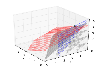
Linear Programming

\[\begin{align} \text{ minimize }&c^Tx+d \\ \text{subject to }&Gx\leq 0 \\ &Ax=b\\ \end{align}\]

In [1]:

import cvxpy as cvp
import cvxopt
import mpl_toolkits.mplot3d.axes3d as p3
import matplotlib.pyplot as plt

In [7]:

x=cvp.Variable(rows=3)
c=np.array([[7,8,9]])
b=np.array([10,8])
G=np.array([[2,1],[3,1],[2,2]])
print 'C:\n',c.T
print 'b:\n',b.T
print 'G:\n',G.T
constraints = [ x>=0,G.T*x <= b]
objective1 = cvp.Minimize(-1*c*x)
p1 = cvp.Problem(objective1, constraints)
p1.solve()
print 'optimal point:\n',x.value

C:
[[7]
 [8]
 [9]]
b:
[10  8]
G:
[[2 3 2]
 [1 1 2]]
optimal point:
[ 2.00e+00]
[ 5.40e-07]
[ 3.00e+00]

In [8]:

fig=plt.figure()
ax = fig.gca(projection='3d')
x = np.arange(0, 5, 0.1)
y = np.arange(0, 5, 0.1)

#Plot first constraints
xx, yy = np.meshgrid(x, y)
z=5-xx-1.5*yy
z[z<0]=np.nan
ax.plot_wireframe(xx,yy,z,  rstride=4, cstride=4, alpha=0.4)

#Plot second constraints
z=4-0.5*xx-0.5*yy
z[z<0]=np.nan
ax.plot_wireframe(xx,yy,z, rstride=2, cstride=2, alpha=0.4,color="red")

#Plot intersection line of two constraints.
yt=1-0.5*x
yt[yt<0]=np.nan
zt=5-x-1.5*yt
zt[zt<0]=np.nan
ax.plot(x,yt,zs=zt)

#Plot level surfaces of the objective function.
def draw_plt(b):
    z=b/9.0-7.0/9*xx-8.0/9*yy
    z[z<0]=np.nan
    if b==40:
        v=1
    else:
        v=2
    ax.plot_wireframe(xx,yy,z, rstride=v, cstride=v, alpha=0.4,color="grey")
map(draw_plt,np.arange(0,45,10))
plt.plot(2,0,zs=[3],marker='d')
ax.set_xlim(0,5)
ax.set_ylim(0,5)
ax.set_zlim(0,5)
ax.set_xlabel('x')
ax.set_ylabel('y')
ax.view_init(elev=30, azim=145)

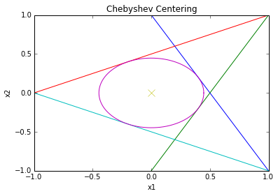
Chebyshev center of polyhedron

Chebyshev center of

\[P=\{x\vert a_i^Tx\leq b_i,i=1\dots m\}\]

is center of largest inscribed ball:

\[B=\{x_c+u \vert \parallel u \parallel_2 \leq r \}\]

$a_i^T x\leq b_i$ for all $x \in B$ iff: $\text{sup } {a_i^T(x_c+u) \vert \parallel u \parallel_2 \leq r }=a_i^Tx_c+r \parallel a_i \parallel_2 \leq b_i$ hence: \(\begin{align} \text{ maximize }&r \\ \text{subject to }&a_i^Tx_c+r\parallel a_i \parallel_2 \leq b_i & i=1\dots m \\ \end{align}\)

In [4]:

from __future__ import division

# From CVXPy examples
# Taken from CVX website http://cvxr.com/cvx/examples/
# Example: Compute and display the Chebyshev center of a 2D polyhedron
# Ported from cvx matlab to cvxpy by Misrab Faizullah-Khan
# Original comments below

# Boyd & Vandenberghe, "Convex Optimization"
# Joelle Skaf - 08/16/05
# (a figure is generated)
#
# The goal is to find the largest Euclidean ball (i.e. its center and
# radius) that lies in a polyhedron described by linear inequalites in this
# fashion: P = { x : a_i'*x <= b_i, i=1,...,m } where x is in R^2

# Create the problem

# variables
radius = cvp.Variable(1)
center = cvp.Variable(2)

# constraints
a1 = cvxopt.matrix([2,1], (2,1))
a2 = cvxopt.matrix([2,-1], (2,1))
a3 = cvxopt.matrix([-1,2], (2,1))
a4 = cvxopt.matrix([-1,-2], (2,1))

b = cvxopt.matrix(1, (4,1))


constraints = [ a1.T*center + np.linalg.norm(a1, 2)*radius <= b[0],
                a2.T*center + np.linalg.norm(a2, 2)*radius <= b[1],
                a3.T*center + np.linalg.norm(a3, 2)*radius <= b[2],
                a4.T*center + np.linalg.norm(a4, 2)*radius <= b[3] ]


# objective
objective = cvp.Maximize(radius)

p = cvp.Problem(objective, constraints)
# The optimal objective is returned by p.solve().
result = p.solve()
# The optimal value
print radius.value
print center.value


# Now let's plot it
x = np.linspace(-2, 2, 256,endpoint=True)
theta = np.linspace(0,2*np.pi,100)

# plot the constraints
plt.plot( x, -x*a1[0]/a1[1] + b[0]/a1[1])
plt.plot( x, -x*a2[0]/a2[1] + b[0]/a2[1])
plt.plot( x, -x*a3[0]/a3[1] + b[0]/a3[1])
plt.plot( x, -x*a4[0]/a4[1] + b[0]/a4[1])


# plot the solution
plt.plot( center.value[0] + radius.value*cos(theta), center.value[1] + radius.value*sin(theta) )
plt.plot( center.value[0], center.value[1], 'x', markersize=10 )

# label
plt.title('Chebyshev Centering')
plt.xlabel('x1')
plt.ylabel('x2')

plt.axis([-1, 1, -1, 1])

plt.show()

0.447213535807
[-9.50e-08]
[-6.87e-18]

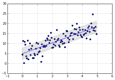
Quadratic Programming

\[\begin{align} \text{ minimize }&1/2x^TP x+q^T x +r\\ \text{subject to }&Gx\leq h \\ &Ax=b\\ \end{align}\]

$P \in S_{+}^n$ and therefore objective is convex.

• Least square is an example of QP:

\[\begin{align} \text{ minimize }&\parallel Ax-b\parallel_2^2 \\ \text{subject to }&Gx\leq h \\ &Ax=b\\ \end{align}\]

\[\begin{align} \parallel Ax-b\parallel_2^2 &= (Ax-b)^T(Ax-b)\\ &=(x^TA^T-b^T)(Ax-b)\\ &=x^TA^TAx-x^TA^Tb-b^TAx+b^Tb \end{align}\]

In [5]:

x=np.arange(0,5,0.05)
y=3*x+np.random.normal(scale=3,size=x.shape[0])+4
A=np.concatenate((np.ones((x.shape[0],1)),x.reshape((x.shape[0],1))),axis=1)
b=y.reshape((x.shape[0],1))
xx=cvp.Variable(rows=2)

objective1 = cvp.Minimize(cvp.quad_form(xx,np.dot(A.T,A))-xx.T*np.dot(A.T,b)-np.dot(b.T,A)*xx)
#
p1 = cvp.Problem(objective1)
p1.solve()
print 'Optimal Point:\n',xx.value

plt.scatter(x,y)
var=np.sqrt(np.var(y.reshape(x.shape[0],1)-np.dot(A,xx.value)))

plt.fill_between(x,np.dot(A,xx.value)[:,0]+var,y2=np.dot(A,xx.value)[:,0]-var
                 , facecolor='grey', alpha=0.2)
plt.plot(x,np.dot(A,xx.value))
plt.grid()

Optimal Point:
[ 4.92e+00]
[ 2.71e+00]