Lecture 0
Introduction to scientific computing with Python
Behzad Tabibian (btabibian@tuebingen.mpg.de) http://btabibian.github.io
J.R. Johansson (robert@riken.jp) http://dml.riken.jp/~rob/
The latest version of this IPython notebook lecture is available at http://github.com/btabibian/scientific-python-lectures.
The other notebooks in this lecture series are indexed at http://btabibian.github.io/notebooks/learnpython/.
The role of computing in science
Science has traditionally been divided into experimental and theoretical disciplines, but during the last several decades computing has emerged as a very important part of science. Scientific computing is often closely related to theory, but it also has many characteristics in common with experimental work. It is therefore often viewed as a new third branch of science. In most fields of science, computational work is an important complement to both experiments and theory, and nowadays a vast majority of both experimental and theoretical papers involve some numerical calculations, simulations or computer modeling.
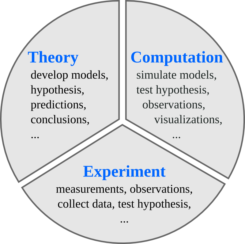
In experimental and theoretical sciences there are well established codes of conducts for how results and methods are published and made available to other scientists. For example, in theoretical sciences, derivations, proofs and other results are published in full detail, or made available upon request. Likewise, in experimental sciences, the methods used and the results are published, and all experimental data should be available upon request. It is considered unscientific to withhold crucial details in a theoretical proof or experimental method, that would hinder other scientists from replicating and reproducing the results.
In computational sciences there are not yet any well established guidelines for how source code and generated data should be handled. For example, it is relatively rare that source code used in simulations for published papers are provided to readers, in contrast to the open nature of experimental and theoretical work. And it is not uncommon that source code for simulation software is withheld and considered a competitive advantage (or unnecessary to publish).
However, this issue has recently started to attract increasing attention, and a number of editorials in high-profile journals have called for increased openness in computational sciences. Some prestigious journals, including Science, have even started to demand of authors to provide the source code for simulation software used in publications to readers upon request.
Discussions are also ongoing on how to facilitate distribution of scientific software, for example as supplementary materials to scientific papers.
References
-
Reproducible Research in Computational Science, Roger D. Peng, Science 334, 1226 (2011).
-
Shining Light into Black Boxes, A. Morin et al., Science 336, 159-160 (2012).
-
The case for open computer programs, D.C. Ince, Nature 482, 485 (2012).
Requirements on scientific computing
Replication and reproducibility are two of the cornerstones in the scientific method. With respect to numerical work, complying with these concepts have the following practical implications:
-
Replication: An author of a scientific paper that involves numerical calculations should be able to rerun the simulations and replicate the results upon request. Other scientist should also be able to perform the same calculations and obtain the same results, given the information about the methods used in a publication.
-
Reproducibility: The results obtained from numerical simulations should be reproducible with an independent implementation of the method, or using a different method altogether.
In summary: A sound scientific result should be reproducible, and a sound scientific study should be replicable.
To achieve these goals, we need to:
-
Keep and take note of exactly which source code and version that was used to produce data and figures in published papers.
-
Record information of which version of external software that was used. Keep access to the environment that was used.
-
Make sure that old codes and notes are backed up and kept for future reference.
-
Be ready to give additional information about the methods used, and perhaps also the simulation codes, to an interested reader who requests it (even years after the paper was published!).
-
Ideally codes should be published online, to make it easier for other scientists interested in the codes to access it.
Tools for managing source code
Ensuring replicability and reprodicibility of scientific simulations is a complicated problem, but there are good tools to help with this:
- Revision Control System (RCS) software.
- Good choices include:
- git - http://git-scm.com
- mercurial - http://mercurial.selenic.com. Also known as
hg. - subversion - http://subversion.apache.org. Also known as
svn.
- Good choices include:
- Online repositories for source code. Available as both private and public repositories.
- Some good alternatives are
- Github - http://www.github.com
- Bitbucket - http://www.bitbucket.com
- Privately hosted repositories on the university’s or department’s servers.
- Some good alternatives are
Note
Repositories are also excellent for version controlling manuscripts, figures, thesis files, data files, lab logs, etc. Basically for any digital content that must be preserved and is frequently updated. Again, both public and private repositories are readily available. They are also excellent collaboration tools!
What is Python?
Python is a modern, general-purpose, object-oriented, high-level programming language.
General characteristics of Python:
- clean and simple language: Easy-to-read and intuitive code, easy-to-learn minimalistic syntax, maintainability scales well with size of projects.
- expressive language: Fewer lines of code, fewer bugs, easier to maintain.
Technical details:
- dynamically typed: No need to define the type of variables, function arguments or return types.
- automatic memory management: No need to explicitly allocate and deallocate memory for variables and data arrays. No memory leak bugs.
- interpreted: No need to compile the code. The Python interpreter reads and executes the python code directly.
Advantages:
- The main advantage is ease of programming, minimizing the time required to develop, debug and maintain the code.
- Well designed language that encourage many good programming practices:
- Modular and object-oriented programming, good system for packaging and re-use of code. This often results in more transparent, maintainable and bug-free code.
- Documentation tightly integrated with the code.
- A large standard library, and a large collection of add-on packages.
Disadvantages:
- Since Python is an interpreted and dynamically typed programming language, the execution of python code can be slow compared to compiled statically typed programming languages, such as C and Fortran.
- Somewhat decentralized, with different environment, packages and documentation spread out at different places. Can make it harder to get started.
What makes python suitable for scientific computing?
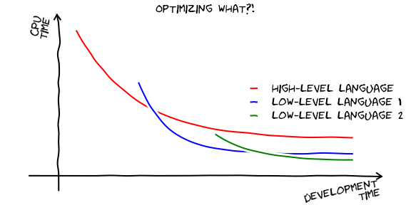
- Python has a strong position in scientific computing:
- Large community of users, easy to find help and documentation.
- Extensive ecosystem of scientific libraries and environments
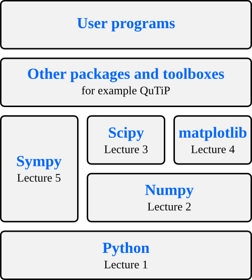
- numpy: http://numpy.scipy.org - Numerical Python
- scipy: http://www.scipy.org - Scientific Python
- scikit-learn: http://scikit-learn.org/stable/ - Machine Learning
- matplotlib: http://www.matplotlib.org - graphics library
- Great performance due to close integration with time-tested and highly optimized codes written in C and Fortran:
- blas, altas blas, lapack, arpack, Intel MKL, …
- Good support for
- Parallel processing with processes and threads
- Interprocess communication (MPI)
- GPU computing (OpenCL and CUDA)
-
Readily available and suitable for use on high-performance computing clusters.
- No license costs, no unnecessary use of research budget.
The scientific python software stack
Python environments
Python is not only a programming language, but often also refers to the standard implementation of the interpreter (technically referred to as CPython) that actually runs the python code on a computer.
There are also many different environments through which the python interpreter can be used. Each environment have different advantages and is suitable for different workflows. One strength of python is that it is versatile and can be used in complementary ways, but it can be confusing for beginners so we will start with a brief survey of python environments that are useful for scientific computing.
Python interpreter
The standard way to use the Python programming language is to use the Python interpreter to run python code. The python interpreter is a program that read and execute the python code in files passed to it as arguments. At the command prompt, the command python is used to invoke the Python interpreter.
For example, to run a file my-program.py that contains python code from the command prompt, use::
$ python my-program.py
We can also start the interpreter by simply typing python at the command line, and interactively type python code into the interpreter.
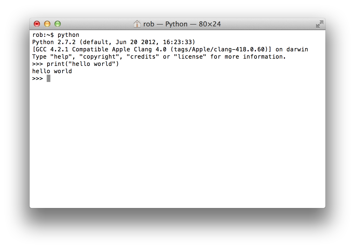
This is often how we want to work when developing scientific applications, or when doing small calculations. But the standard python interpreter is not very convenient for this kind of work, due to a number of limitations.
IPython
IPython is an interactive shell that addresses the limitation of the standard python interpreter, and it is a work-horse for scientific use of python. It provides an interactive prompt to the python interpreter with a greatly improved user-friendliness.
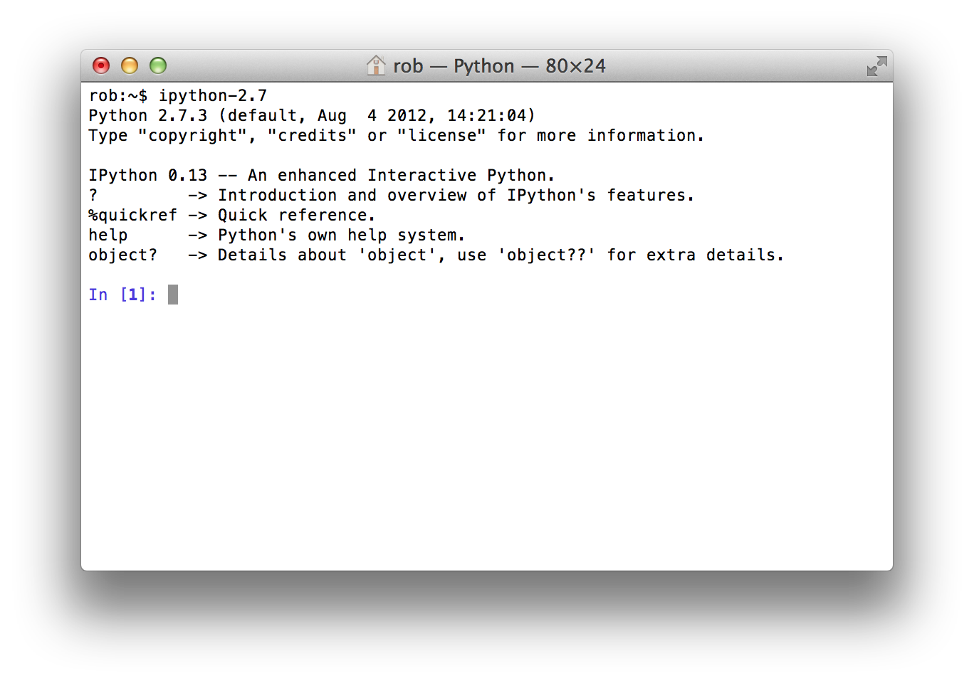
Some of the many useful features of IPython includes:
- Command history, which can be browsed with the up and down arrows on the keyboard.
- Tab auto-completion.
- In-line editing of code.
- Object introspection, and automatic extract of documentation strings from python objects like classes and functions.
- Good interaction with operating system shell.
- Support for multiple parallel back-end processes, that can run on computing clusters or cloud services like Amazon EC2.
Jupyter notebook (formerly IPython)
Jupyter notebook is an HTML-based notebook environment for Python, similar to Mathematica or Maple. It is based on the IPython shell, but provides a cell-based environment with great interactivity, where calculations can be organized documented in a structured way. The notes you are reading are produced using this tool. You can download these notebooks from here.
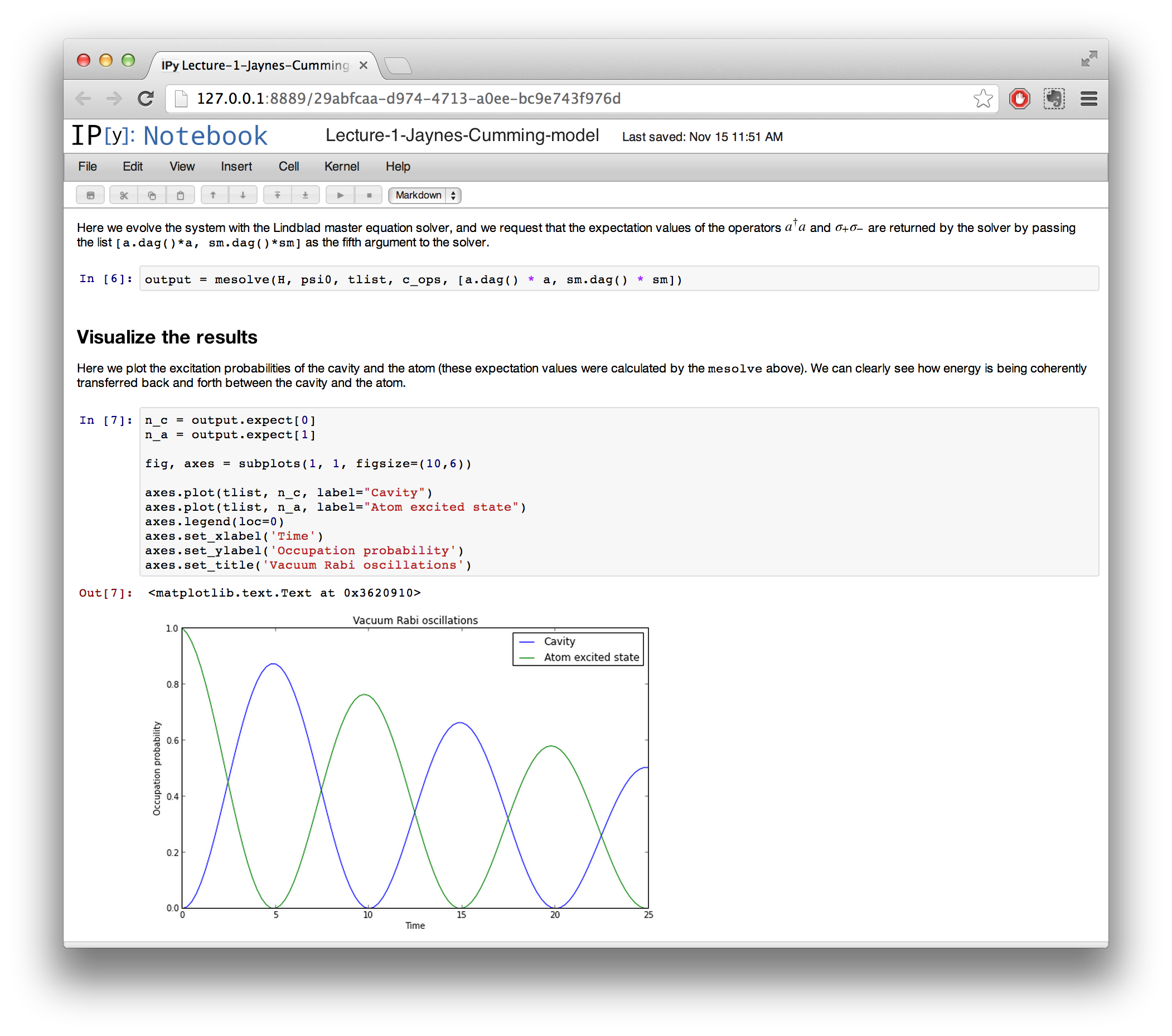
Although using the a web browser as graphical interface, IPython notebooks are usually run locally, from the same computer that run the browser. To start a new IPython notebook session, run the following command:
$ ipython notebook
from a directory where you want the notebooks to be stored. This will open a new browser window (or a new tab in an existing window) with an index page where existing notebooks are shown and from which new notebooks can be created.
Spyder
Spyder is a MATLAB-like IDE for scientific computing with python. It has the many advantages of a traditional IDE environment, for example that everything from code editing, execution and debugging is carried out in a single environment, and work on different calculations can be organized as projects in the IDE environment.
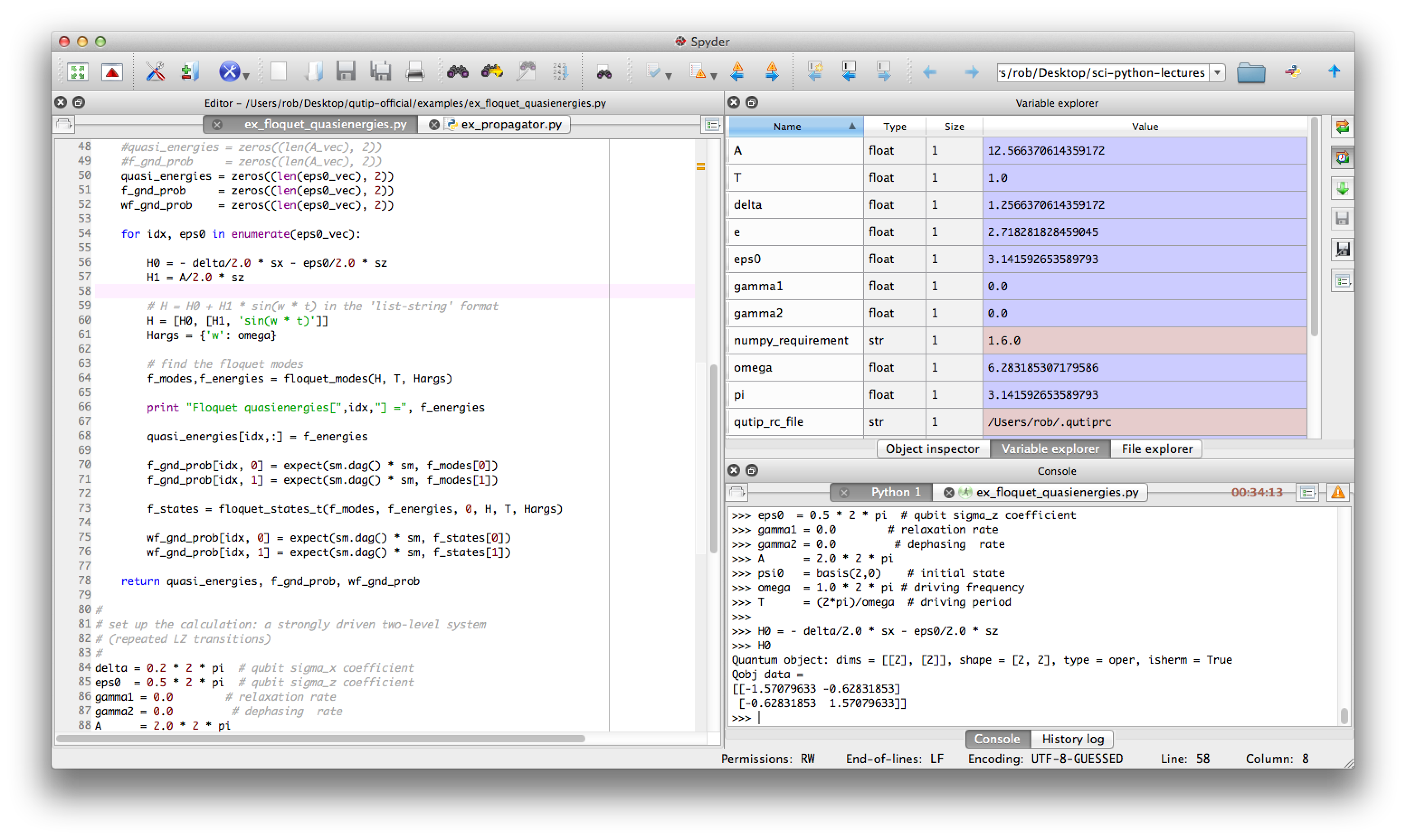
Some advantages of Spyder:
- Powerful code editor, with syntax high-lighting, dynamic code introspection and integration with the python debugger.
- Variable explorer, IPython command prompt.
- Integrated documentation and help.
Versions of Python
There are currently two versions of python: Python 2 and Python 3. Python 3 will eventually supercede Python 2, but it is not backward-compatible with Python 2. A lot of existing python code and packages has been written for Python 2, and it is still the most wide-spread version. For these lectures either version will be fine, but it is probably easier to stick with Python 2 for now, because it is more readily available via prebuilt packages and binary installers.
To see which version of Python you have, run
$ python --version
Python 2.7.3

$ python3.2 --version
Python 3.2.3
Several versions of Python can be installed in parallel, as shown above.
Installation
The most convinient way to install necessary packages for this course is to use Annaconda’s distribution. This distrubition contains almost all the packages needed for this course.
Visit http://continuum.io/downloads to obtain the latest version of this distribution for your platform. You may download and install any version after 2.1 but make sure you are not installing older versions.
Linux
In Ubuntu Linux, download bash script from the download page of annaconda. Run following command from where you downloaded to file:
$ sudo bash Anaconda-2.2.0-Linux-x86_64
MacOS X
Annaconda provides a Graphical Installer which provides all neccessary packages.
Windows
Similar to Mac, you can download the installer for Windows from Annaconda download page.
Check your installation
After installing one of the above distributions you can check your installation by opening a new terminal window and type following commands:
$ ipython --version

3.0.0

$ ipython

In [1]: import numpy as np

In [2]: import matplotlib.pyplot as plt
If you obtained a copy of this notebook you can run the notebook by starting an IPython session, discussed above, and run the notebook and compare your environment with the one used to produce the outputs at the end of this notebook.
Further reading
- Python. The official Python web site.
- Python tutorials. The official Python tutorials.
- Think Python. A free book on Python.
Python and module versions
Since there are several different versions of Python and each Python package has its own release cycle and version number (for example scipy, numpy, matplotlib, etc., which we installed above and will discuss in detail in the following lectures), it is important for the reproducibility of an IPython notebook to record the versions of all these different software packages. If this is done properly it will be easy to reproduce the environment that was used to run a notebook, but if not it can be hard to know what was used to produce the results in a notebook.
To encourage the practice of recording Python and module versions in notebooks, I’ve created a simple IPython extension that produces a table with versions numbers of selected software components. I believe that it is a good practice to include this kind of table in every notebook you create.
To install this IPython extension, run:
1
2
# you only need to do this once
%install_ext http://raw.github.com/jrjohansson/version_information/master/version_information.py
Installed version_information.py. To use it, type:
  %load_ext version_information
Now, to load the extension and produce the version table
1
2
3
%load_ext version_information

%version_information numpy, scipy, matplotlib, sympy
| Software | Version |
|---|---|
| Python | 2.7.8 64bit [GCC 4.4.7 20120313 (Red Hat 4.4.7-1)] |
| IPython | 3.0.0 |
| OS | Linux 3.13.0 45 generic x86_64 with debian jessie sid |
| numpy | 1.9.1 |
| scipy | 0.14.0 |
| matplotlib | 1.3.1 |
| sympy | 0.7.5 |
| Mon Apr 13 10:39:11 2015 CEST | |
