02-Convexity-Preserving-Operations

This is the second notebook of the series going through Convex Optimizaion. The topics here are following MOOC Convex Optimization course by Stephen Boyd at Stanford.

---

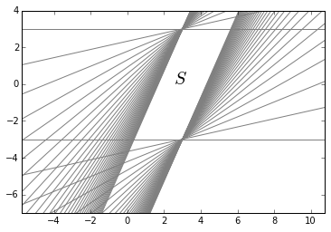
Intersection:

If $S_1$, $S_2$ are convex then:

$S_1\cap S_2$ is convex.

Example:

The example below is a set constructed by intersecting many halfspaces.

In [40]:

plt.axis('equal')
def plot(m):
    plt.plot(np.arange(-10,10)+v[0],np.arange(-10,10)*m+v[1],color='grey')
v=[3,3]
map(plot,np.log(np.arange(1,10,0.25)))
v=[3,-3]
map(plot,np.log(np.arange(1,10,0.25)))
plt.xlim(-2,7)
plt.ylim(-7,4)
plt.text(2.5,0,'$S$',fontdict={'fontsize':20})
plt.legend()

Afine functions:

$f: R^n \rightarrow R^m$ is affine if $f(x)=Ax+b$, where $A \in R^{m \times n}$ and $b\in R^m$, (sum of a linear function and a constant)

• Suppose $S\subseteq R^n$ is convex and $f$ an affine function, Then $f(S)$ is convex.

• If $f: R^k \rightarrow R^n$ is an affine function, then inverse image of $S$ under $f$:$f^{-1}(S) = {x\mid f(x)\in S}$ is convex.

Examples:

• Scaling and translations are convex preserving:

  if $S\subseteq R^n$ is convex, $\alpha \in R$ an $a\in R^n$, then the sets $\alpha S$ and $S+a$ are convex:

  $\alpha S=\{\alpha x\mid x\in S\}$, $S+a=\{x+a\mid x \in S\}$

• Projection of a convex set onto some of its coordinates is convex.:

  if $S\subseteq R^m \times R^n$ is convex, then

  $T=\{x_1 \in R^m\mid (x_1,x_2) \in S \text{ for some } x_2 \in R^n\}$

  is convex.

• The sum of two sets is defined as:

  \[S_1+S_2=\{x+y\mid x\in S_1,s_2\in S_2\}\]

  If $S_1$ and $S_2$ are convex, then $S_1+S_2$ are convex.

  To see why we note that:

  if $S_1$ and $S_2$ are convex so is Cartesian product:

  $S_1\times S_2=\{(x_1,x_2)\mid x_1\in S_1, x_2 \in S_2\}$

  The image of this set under the linear funciton $f(x_1,x_2)=x_1+x_2$ is the sum $S_1+S_2$.

Linear Fractionals and perspective functions:

The perspective function:

\[\begin{align} P: R^{n+1}\rightarrow r^n\\ \textbf{dom }P=R^n\times R_{++}&,R_{++}=\{x\in R\mid x>0\}\\ P(z,t)=z/t\\ \end{align}\]

This function scales or normalizes vectors by last component and then drops normalizer.

• If $C \subseteq \textbf{dom} P$ is convex, then its image:

  \[P(C)=\{P(x)\mid x\in C\}\]

  is convex.

Suppose \(x = (\tilde{x},x_{n+1}),y = (\tilde{y},y_{n+1}) \in R^{n+1}\) and \(x_{n+1}>0, y_{n+1}> 0, \text{ then for }0 \leq \theta \leq 1\) we have:

\(\begin{align} P(\theta x+(1-\theta)y)&=\frac{\theta \tilde{x}+(1-\theta)\tilde{y}}{\theta x_{n+1}+(1-\theta)y_{n+1}}\\ &=\frac{\theta x_{n+1}}{\theta x_{n+1}+(1-\theta)y_{n+1}}\frac{\tilde{x}}{x_{n+1}}+\frac{(1-\theta) y_{n+1}}{\theta x_{n+1}+> (1-\theta)y_{n+1}}\frac{\tilde{y}}{y_{n+1}}\\ &=\mu P(x)+(1-\mu)P(y)\\ \end{align}\) where \(\mu=\frac{\theta x_{n+1}}{\theta x_{n+1}+(1-\theta) y_{n+1}} \in [0,1]\) and monotonic. This establishes the convexity preserving of $P$. If $C$ is convex with $C \subseteq \textbf{dom} P$ from above we have that the line segment $[P(x),P(y)]$ is in $P(C)$.

• The inverse image of a convex set under the perspective function is also convex:

  if $C\subseteq R^n$ is convex, then:

  $P^{-1}(C)=\{(x,t)\in R^{n+1}\mid x/t\in C,t>0\}$

  is convex.

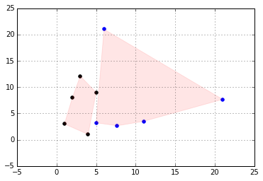
Linear-fractional functions:

A linear-fractional function is formed by composing the perspective function with and affine function:

suppose $g:R^n\rightarrow R^{m+1}$ is affine:

\[\begin{align} g(x)=\begin{bmatrix} A\\ c^T \end{bmatrix} x+\begin{bmatrix} b\\ d \end{bmatrix}\\ \end{align}\]

Where $A \in R^{m \times n}$,$b\in R^m$,$c \in R^n$ and $d \in R$. The function $f:R^n \rightarrow R^m$ given by $f=p \circ g$:

\begin{align} f(x)=(Ax+b)/(c^Tx+d), \textbf{dom}f={x \mid c^Tx+d>0}
\end{align}

If $c=0$ and $d>0$, the domain of $f$ is $R^n$ and $f$ is an affine function.

linear-fractional functions are convex preserving.

In [131]:

import matplotlib.patches as mpatches
plt.grid()
C=np.array([[1,3],[2,8],[3,12.1],[5,9],[4,1]])
region=plt.Polygon(C,alpha=0.1,color='r')
plt.gca().add_patch(region)
plt.scatter(C[:,0],C[:,1],color='k',label='$C$')
A=np.array([[1,0],[0,1]])
b=np.array([20,20])
c=np.array([[1,0],[0,1]])
d=np.array([0,0])
den=np.dot(A,C.T).T+np.tile(b,(C.shape[0],1))
par=np.dot(c,C.T).T+np.tile(d,(C.shape[0],1))
c_=den/par
region=plt.Polygon(c_,alpha=0.1,color='r')
plt.gca().add_patch(region)
plt.scatter(c_[:,0],c_[:,1],color='b',label='$C\'$')

<matplotlib.collections.PathCollection at 0x11035f650>

---

Generalized inequalities

Proper cones and generalized inequalities

A cone $K \subseteq R^n$ is called a propor cone of it satisfies following:

• K is convex
• K is closed.
• K is solid, it has nonempty interior.
• K is pointed, it has no line or $x\in K, -x \in K \Rightarrow x=0$

Generalized inrquality is defined over a proper cone:

\begin{align} x\preceq_K y \iff y-x\in K. \end{align} and for the strict ordering:

\begin{align} x\prec_K y \iff y-x\in \textbf{int }K. \end{align}

Examples

• if $K=R_+$ then partial ordering $\prec_K$ is the usual $\leq$ on R.

  $x\preceq_{R_+} y \iff y_i-x_i\geq 0$.

• positive semidefinite cone $K=S_{+}^n$.

  $X\preceq_{S_{+}} Y \iff Y-X \text{ is postive semidifnite}$.

Minimum and Minimal elements

• $x\in S$ is the minimum element of $S$ with respect to $\preceq_k$ if:

  $y\in S \Rightarrow x \preceq_k y$.

• $x\in S$ is the minimal element of $S$ with respect to $\preceq_k$ if:

  $y\in S, y \preceq_k x \Rightarrow x = y$.